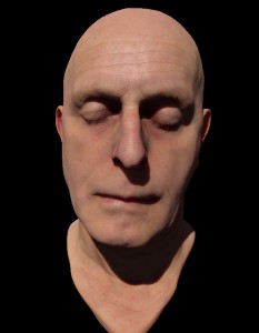
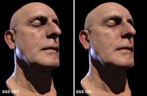
 I’ve recently decided to look into supporting subsurface scattering in my playground rendering engine Helix. It’s not the first time I’ve dabbled in the subject, but not being limited to crappy platforms I could push things a bit further. It’s a well researched and oft written about topic, so I’ve been reluctant to write up on the results of my implementation, especially seeing how heavily it’s based on these writings. But then I reflected back at why I started this blog in the first place: sharing a learning process. Not everyone likes reading papers so an implementation overview to go along with them might be helpful. The implementation I’ll show is simplified and slightly different to what you’ll find in the source material:
- Eugene d’Eon: GPU Gems 3 Chapter 14: Advanced Techniques for Realistic Real-Time Skin Rendering
- Jorge Jimenez and Diego Gutierrez’ article in GPU Pro: Screen-Space Subsurface Scattering
- Nicolas Schulz: The Rendering Technology of Ryse (I discovered relatively late how similar my solution was to this, which is both a bummer and encouraging ;) )
I really recommend checking out these links if you have more than a passing interest in the subject (or to verify that I really can’t take credit for much in this post!). Finally, Gaussian convolutions are an important concept in what follows so if you’re hazy on the subject, read up on Gaussian blurs and how to implement them on compute shaders (explained in any decent DirectX 11 intro book, or here).
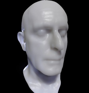
The head model used in the screenshots is provided by Ten24 here.
Introduction
Simply put, light can do two things when hitting an object. Either it reflects (specular reflections) or it enters the object. In the latter case, it bounces around inside for a bit before re-emerging at the surface (diffuse scattering). The properties of the material define how far the light is likely to travel before exiting. This distance is often so small that we traditionally assume that it emerges at the same exact point it enters. This distance can however be quite large for translucent materials and this assumption fails to result in convincing images; surfaces look to harsh or claylike.
As light passes through, parts of its spectrum get absorbed. In other words, light tends to discolour more the further it travels underneath the surface. The function of discolouration over distance is expressed using a diffusion profile (refer to d’Eon). Some materials consist of several layers that absorb light differently (consider the layers of skin: oil, epidermis, dermis) so the diffusion profile can get quite complex. d’Eon uses the sum of 6 Gaussians to approximate the profile for skin, and Jimenez further reduces it to 4 (which can be implemented as 3, more on that later). Again, I suggest reading those articles if you haven’t yet, I don’t want to repeat them too much.
Translucency results in a couple of visible effects, depending on where the light enters and exits the surface relative to the viewer. We’ll deal with each in separate ways.
- Back-lit transmittance: Light enters the back side of an object and exits from the front.
- Same-side surface scattering: Light exits on the same side of an object.
For my own implementation, I put forth the following goals:
- Both back-lighting and same-side surface scattering should be supported.
- It needs to work nicely with Helix’s deferred rendering pipeline. This meant working in screenspace.
- Support multiple material profiles: not only skin, but wax, marble, jade, sticky white substances, …
- While not being limited to it, it should be able to represent believable skin
Render pipeline
To get started, I’ll detail the GBuffer layout and the render pipeline I settled on (even if it’s something I keep changing constantly ;) ):
| 0 | Depth | Stencil | ||
| 1 | Albedo R | Albedo G | Albedo B | Emission |
| 2 | Packed normal X | Packed normal Y | Translucency | Extended Material Profile ID |
| 3 | Metallicness | Normal specular reflectivity | Roughness | TBD |
Layer 3 is irrelevant for subsurface scattering since it’s only used for specular reflections. In case you’re interested, it’s not unlike Unreal Engine 4’s approach to specular representations.
- Translucency: The amount of back-lighting allowed to pass through the surface.
- Extended material profile: Contains an ID of the surface type. For example: 0 = default, 1 = skin, 2 = marble, … More on that later.
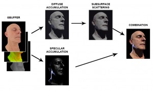
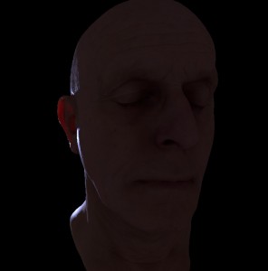
Subsurface scattering does not affect specular reflections, so we’ll need to accumulate the lighting using separate HDR light accumulation buffers for diffuse and specular (the R11G11B11_FLOAT texture format worked well for me). Our diffuse target does not have albedo applied yet. The render pipeline is as follows:
- Render material properties to the GBuffer.
- Render lights to diffuse + specular accumulation buffers (lighting includes transmittance)
- Perform subsurface scattering
- Combine lighting and apply albedo: light = (diffuse + emission) * albedo + specular
- Post-processing (bloom, tone mapping, …)
Why doesn’t the diffuse accumulation buffer have albedo applied, you ask? It probably doesn’t matter all that much, but my reasoning is as follows: albedo maps are usually generated from scans in evenly lit situations and as such already exhibit a degree of subsurface scattering (that’s why they are coloured the way they are in the first place!). Similarly, maps created by artists tend to mimic this look as well.
Extended Material Profiles
To support different material types, we store an “extended material profile” index in the GBuffer. This will be used to access a structured buffer object in the shaders. Each entry is of type ExtendedMaterialProfile which contains details about the (sub)surface properties. Since these properties are per material type and don’t vary per pixel (which is of course a simplification of reality) we don’t need to store all properties in the GBuffer, which would be prohibitively expensive. This construct is not necessarily only used for subsurface scattering but could be extended for other effects. The ExtendedMaterialProfile struct is defined in the shader as follows:
{
// same-side scattering properties
int enableSubsurfaceScattering;
uint numGaussians;
float subsurfaceRadius;
float3 originalBlendFactors;
float3 subsurfaceBlends[MAX_GAUSSIANS];
float4 subsurfaceGaussianExponents;
// back-lit transmittance properties
int enableDistanceBasedTransmittance;
float3 transmittanceCoefficient;
};
What every property means will be explained as we go.
Back-lit Transmittance
For default materials, we handle back-lit transmittance in a very traditional way: we invert the normal, calculate lighting for that and add it to the calculated light:
transmittanceCoefficient is a simple colour value to modulate the amount of light transmitted. This approach is useful for thin surfaces such as leaves or paper. For objects with more volume we need to calculate (or rather: estimate) how far light has travelled through the object in order to know how much of it is absorbed. This is in fact the same as we did way back in Away3D Broomstick.
To recap: we get the depth value from the shadow map and use that to calculate the position of the occluder (not sure how?). We can use the distance between the occluder and the shaded point as an estimate of how far the light has travelled through the object. Unfortunately, this approach requires lights to have shadow maps associated with them. Helix simply ignores distance-based transmittance for those that don’t. You may also want to consider storing linear depth values for point and spot lights to prevent reduced precision further away from the light.
Armed with this distance value, I’ve found that using the Beer-Lambert law for transmittance allows for convincing enough results for common cases. For each colour channel, the transmitted ratio of light for distance ![]() is as follows:
is as follows:
![]()
Again, we simply use the inverted normal to get an approximation of light hitting the other side of the surface. The total diffuse lighting for the pixel will be:
Louis Bavoil suggests a nice artist-friendly way to calculate the transmittanceCoefficient value for a measured colour at a given distance, which is implemented on the C++ side of the ExtendedMaterialProfile in the following convenience method:
{
enableDistanceBasedTransmittance = 1;
transmittanceCoefficient = -Ln(measuredColor) / measureDistance;
}
The enableDistanceBasedTransmittance property dictates which approach is used. For leaves, we’d set it to 0, for skin we’d want 1. The amount of transmitted light is modulated using a transmittance mask, the values of which are written to the GBuffer.
You could also use the diffusion profile to calculate the transmittance (which is something I’ll probably experiment with at some point). For now, this is faster and quite acceptable.
Same-side subsurface scattering
This aspect deserves a bit more finesse. After all, it’s what gives skin its organic fleshy look and we want the implementation to be solid enough to support this believably. As humans, we’re very attuned to recognizing others as humans; we can easily spot fake ones based on small perceptional errors. We’ll base ourselves on Jimenez’ approach of using 4 Gaussians and we’ll treat other diffusion profiles the same way. Remember what Gaussian distributions look like for variance ![]() :
:
![]()
![]()
![]()
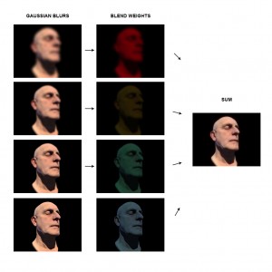
Jimenez’ approach can be thought of as performing 4 Gaussian blurs on the image and blending them together with different weights per colour channel. Note that the sum of all blend weights must be 1 for every colour channel or energy would be lost or gained when compositing.
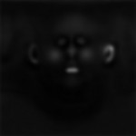
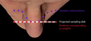
Talking about Gaussian blurs; some implementations do exactly that. By using a fixed sample count the samples’ weights can be precomputed (the total blended sum-of-gaussians, that is). The sampling disk around the centre pixel is rotated to more closely match the orientation of the surface and projected to screen space. This way, a somewhat correct range is sampled. However, using the distance of the sampling points’ on the sampling disk as weights for the Gaussian convolution assumes that all sampled points are evenly spaced. This does not necessarily match with what’s on screen. Take a look at a top-down view of such a sampling:
As you can see, the real distances to the central point are quite different. This can lead to an over-contribution of samples at strongly varying surfaces, manifesting in halos. In my implementation, I used the depth buffer to reconstruct view space positions to get actual view-space distances. While still not a correct estimate of how far the light has travelled underneath the surface, it’s a better approximation. However, it also means that the samples aren’t necessarily evenly distributed with respect to the Gaussian curve. This is really only a problem at discontinuities and is in my opinion less objectionable than halo artefacts. Since our sampling weights are not known beforehand, we need to manually normalize the calculation. This means we’ll need to sum all calculated weights and use it to ‘average out’ the total.
There’s some extra benefits to this approach. Because we’re manually normalizing the total, we don’t have to use a fixed sample count: we can limit the sampling to exactly the pixels we need. A traditional Gaussian convolution with precomputed weights would require us to sample ![]() points, even if the radius is less than
points, even if the radius is less than ![]() pixels. This doesn’t really contribute any new info (sampling 11 points across 4 pixels is a waste). Similarly, when the radius exceeds
pixels. This doesn’t really contribute any new info (sampling 11 points across 4 pixels is a waste). Similarly, when the radius exceeds ![]() , we can now add the contribution for every pixel, increasing the quality.
, we can now add the contribution for every pixel, increasing the quality.
A smaller bonus is that the Gaussian calculation can be a bit simplified. The gaussian functions themselves don’t need to be scaled with a normalization factor as it will be implicit in the total (ie: we can drop the ![]() factor in the Gaussian formula above).
factor in the Gaussian formula above).
Using the real distance and a manual normalization isn’t without its drawbacks, however. Most obviously, the position needs to be reconstructed from the depth buffer. This means extra texture fetches and calculations. Furthermore, we can’t precompute the sum-of-Gaussians and store them in a lookup texture. Every Gaussian will need to be calculated separately, and a total weight should be counted for each, so that each curve can be normalized individually. If we wouldn’t do this, we’d get an incorrect balance between the layers.
Finally, Jimenez observes that the first Gaussian for skin has such a small variance that it usually wholly falls within a single pixel. This means that we can just calculate 3 Gaussians and the value from the original diffuse buffer’s value.
Separability
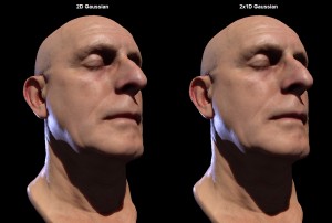
2D Gaussians are separable: it’s identical to a horizontal 1D Gaussian followed by a vertical one, reducing the amount of samples necessary to ![]() instead of
instead of ![]() . However, this is not the case with depth-dependent Gaussians, nor the sum of several. However, ignoring this and merging everything in 2 passes anyway (instead of doing it in up to 8) doesn’t result in a noticeable difference.
. However, this is not the case with depth-dependent Gaussians, nor the sum of several. However, ignoring this and merging everything in 2 passes anyway (instead of doing it in up to 8) doesn’t result in a noticeable difference.
I needed to use the histogram in Photoshop with the “difference” blend layer to verify that there was in fact a slight difference, mainly due to the wider red Gaussian. In any case, it gets my pseudo-separable stamp!
Performing 1D convolutions sampling only at pixel centres is pretty efficient using compute shaders, meaning we can get higher fidelity and less noise than using a fragment shader using jittered samples.
Implementation
Returning to the ExtendedMaterialProfile struct, we can now explain what the other properties mean:
- enableSubsurfaceScattering; Indicates whether or not subsurface scattering should be performed for this material.
- numGaussians: the amount of Gaussians. 3 for skin, for example.
- subsurfaceRadius: the sample radius in meters of the largest Gaussian, derived from the variances.
- originalBlendFactors: the amount of unblurred diffuse lighting that is blended in. This is used to replace the smallest Gaussian for skin.
- subsurfaceBlends: the amount of blending for each Gaussian layer. Summed all together with originalBlendFactors, it needs to form 1 for each channel.
- subsurfaceGaussianExponents: The exponents used to calculate the Gaussian weights (
 from the Gaussian formula above)
On the C++ side, another convenience method is provided to set the subsurface properties:
{
float3 total(0.0, 0.0, 0.0);
enableSubsurfaceScattering = 1;
this->numGaussians = numGaussians;
for (unsigned int i = 0; i < numGaussians; ++i) {
// calculate the total blend weights of the gaussians, used to automatically set the amount of unblurred light
total += blendWeights[i]; subsurfaceBlends[i] = blendWeights[i];
// gaussian normal distribution
subsurfaceGaussianExponents[i] = -1.0f / (2.0f * variances[i]);
// use standard deviation as a radius estimate
// Gaussian is expressed in terms of millimeters, radius needs to be in meters, so divide by 1000.0f!
float radius = Sqrt(variances[i]) / 1000.0f;
if (radius > subsurfaceRadius)
subsurfaceRadius = radius;
}
// the amount of the original unblurred diffuse is just as much so that all blend weights sum to 1
originalBlendFactors = 1.0 - total;
}
We’re using compute shaders to perform the 1D convolutions, so we can efficiently pre-fetch the texture samples and calculate the view-space positions in faster group-shared memory. An overview of the compute shader:
- Gather and precompute everything required for the current compute shader thread group, so we don’t need to do this per sample:
- diffuse radiance, sampled from accumulation buffer
- view-space position, derived from depth buffer
- Retrieve the extended material ID.
- Project the sample radius using the camera to get a radius approximation in screen space.
- Loop over all samples falling within the projected sample radius.
- Calculate distance to central pixel
- Calculate Gaussian weight for pixel
- Add weighted radiance sample
- Add weight to total
- “Average out” total radiance using total weight count.
The code below should make this a bit clearer. It’s for the horizontal Gaussians only, but the vertical is nearly identical:
#define MAX_RADIUS 32
#define MAX_GAUSSIANS 4
struct ExtendedMaterialProfile
{
int enableSubsurfaceScattering; // whether or not to use subsurface scattering (0 or 1)
uint numGaussians; // the amount of gaussians to approximate the diffusion profile
float subsurfaceRadius; // the radius in meters of the largest Gaussian
float3 originalBlendFactors; // the ratio of the original unblurred texture to add
float3 subsurfaceBlends[MAX_GAUSSIANS]; // the blend weights for each gaussian
float4 subsurfaceGaussianExponents; // The constant factor of the Gaussian exponents: -1.0f / (2.0f * variances[i]);
// We store the exponents for all 4 in a single float4 for convenience (see code)
int enableDistanceBasedTransmittance; // whether or not to use distance-based transmittance scattering (0 or 1, unused here but used in the lighting shader)
float3 transmittanceCoefficient; // if enableDistanceBasedTransmittance = 0, this is just the colour of the backlit light, otherwise, it's the density of the beer-law exponent
};
cbuffer cameraData
{
float4x4 projectionMatrix; // the local projection matrix
float4 viewFrustumVectors[4]; // contains the view frustum vectors for each edge going from the near to far plane, scaled so that z == 1, in clockwise order starting top-left
float2 renderTargetResolution; // the size of the render target
};
Texture2D<float3> diffuseSource;
Texture2D<float> gbufferDepth;
Texture2D<float4> gbufferNormalMaterial;
StructuredBuffer<ExtendedMaterialProfile> extendedMaterialProfiles;
RWTexture2D<float3> diffuseTarget;
groupshared float3 radianceSamples[2 * MAX_RADIUS + NUMTHREADS];
groupshared float3 positionSamples[2 * MAX_RADIUS + NUMTHREADS];
// Retrieve the view vector for a given pixel coordinate.
float4 GetViewVector(uint2 coord)
{
// turn coords into a uv ratio for interpolation
float2 uv = coord / renderTargetResolution;
// Uses standard trilinear interpolation
float4 top = lerp(viewFrustumVectors[0], viewFrustumVectors[1], uv.x);
float4 bottom = lerp(viewFrustumVectors[3], viewFrustumVectors[2], uv.x);
return lerp(bottom, top, uv.y);
}
// Unproject a value from the depth buffer to the Z value in view space.
// Multiply the result with an interpolated frustum vector to get the actual view-space coordinates
// Refer to https://www.derschmale.com/2014/01/26/reconstructing-positions-from-the-depth-buffer/ for more info on this:
float DepthToViewZ(float depthValue)
{
return projectionMatrix[3][2] / (depthValue - projectionMatrix[2][2]);
}
// returns the view-space position for the point at the given pixel
// coord: the pixel coordinate to sample the depth at
// viewDir: the view direction (with z == 1) matching the pixel coordinate
// Refer to https://www.derschmale.com/2014/01/26/reconstructing-positions-from-the-depth-buffer/ for more info on this
float3 GetViewPosition(uint2 coord, float3 viewDir)
{
return viewDir * DepthToViewZ(gbufferDepth[coord]);
}
[numthreads(NUMTHREADS, 1, 1)]
void main(uint3 dispatchThreadID : SV_DispatchThreadID, uint3 groupThreadID : SV_GroupThreadID)
{
// Store all radiance samples and view-space positions in groupshared memory.
// See Gaussian blur example at: http://amd-dev.wpengine.netdna-cdn.com/wordpress/media/2012/10/Efficient%20Compute%20Shader%20Programming.pps
float3 viewDir = GetViewVector(dispatchThreadID.xy).xyz;
float3 frustumDiff = float3((viewFrustumVectors[2].x - viewFrustumVectors[3].x) / renderTargetResolution.x, 0.0, 0.0);
float3 centerSample = diffuseSource[dispatchThreadID.xy];
float3 viewPosition = GetViewPosition(dispatchThreadID.xy, viewDir);
// the central pixel is placed in "groupThreadID.x + MAX_RADIUS"
radianceSamples[groupThreadID.x + MAX_RADIUS] = centerSample;
positionSamples[groupThreadID.x + MAX_RADIUS] = viewPosition;
if (groupThreadID.x < MAX_RADIUS) {
float2 coord = dispatchThreadID.xy - uint2(MAX_RADIUS, 0);
radianceSamples[groupThreadID.x] = diffuseSource[coord];
positionSamples[groupThreadID.x] = GetViewPosition(coord, viewDir - frustumDiff * MAX_RADIUS);
}
else if (groupThreadID.x >= NUMTHREADS - MAX_RADIUS) {
float2 coord = dispatchThreadID.xy + uint2(MAX_RADIUS, 0);
radianceSamples[groupThreadID.x + 2 * MAX_RADIUS] = diffuseSource[coord];
positionSamples[groupThreadID.x + 2 * MAX_RADIUS] = GetViewPosition(coord, viewDir + frustumDiff * MAX_RADIUS);
}
// Wait for all data to be ready
GroupMemoryBarrierWithGroupSync();
// fetch material profile ID, stored in alpha channel of the normal/material GBuffer texture
float4 normalMaterialData = gbufferNormalMaterial[dispatchThreadID.xy];
ExtendedMaterialProfile profile = extendedMaterialProfiles[normalMaterialData.w * 255];
// if no subsurface scattering is required, simply output the original sample
if (!profile.enableSubsurfaceScattering) {
diffuseTarget[dispatchThreadID.xy] = centerSample;
return;
}
// project the sample radius
float w = viewPosition.z * projectionMatrix[2][3] + projectionMatrix[3][3];
float radiusProjection = projectionMatrix[1][1] / w * renderTargetResolution.x * .25;
int sampleRadius = profile.subsurfaceRadius * radiusProjection;
// sample radius too small, would just convolute a single pixel, so just return that immediately
if (sampleRadius < 1) {
diffuseTarget[dispatchThreadID.xy] = centerSample;
return;
}
// make sure we don't go out of bounds (usually when getting the camera very close)
sampleRadius = min(sampleRadius, MAX_RADIUS - 1);
float4 totalWeights = 0;
// stores all 4 blurs in a single var
float4x3 totals = 0;
for (int i = -sampleRadius; i <= sampleRadius; ++i) {
// Remember the central pixel is placed in "groupThreadID.x + MAX_RADIUS"
int index = groupThreadID.x + MAX_RADIUS + i;
float3 dir = positionSamples[index] - viewPosition;
// Calculate the squared distance and convert from meters^2 to millimeters^2 (squared, so multiply by 1000^2)
float distSqr = dot(dir, dir) * 1000000.0f;
// Calculate all 4 Gaussian weights
float4 weights = exp(distSqr * profile.subsurfaceGaussianExponents);
totalWeights += weights;
// add the sample to each layer with their respective Gaussian weight
[unroll]
for (int j = 0; j < MAX_GAUSSIANS; ++j)
totals[j] += weights[j] * radianceSamples[index];
}
// start with the amount of original diffuse light that we specified
float3 total = centerSample * profile.originalBlendFactors;
// add blended blurred results
[unroll]
for (int j = 0; j < MAX_GAUSSIANS; ++j)
total += totals[j] / totalWeights[j] * profile.subsurfaceBlends[j].xyz;
diffuseTarget[dispatchThreadID.xy] = total;
}
Conclusion
By adding different configurations to the StructuredBuffer in the shader, you can easily support different materials per shader. Skin is created using Jimenez’ settings:
float3 blends[3] = { float3(.1158f, .3661f, .3439f), float3(.1836f, .1864f, .0f), float3(.46f, .0f, .0402f) };
profile.SetSubsurfaceScattering(3, blends, variances);
profile.SetTransmittanceCoefficientByDistance(float3(.94f, .14f, .14f), .0002f);
Other materials can be created, such as wax:
float3 blends[4] = { float3(.0544f, .1245f, .2177f), float3(.2436f, .2435f, .1890f), float3(.3105f, .3158f, .3742f), float3(.3913f, .3161f, .2189f) };
profile.SetSubsurfaceScattering(4, blends, variances);
profile.SetTransmittanceCoefficientByDistance(float3(.3913f, .3161f, .2189f), .1f);
I’ll leave you with an observation. Recently, I’ve been watching Breaking Bad (yeah, I’m way behind on the cool stuff). Don’t you think Cranston has the best distribution profile going on?



Hi David,
Very nice work!
Thanks for sharing!
I’m interested in the gaussian blur, did you find the compute shader for the Gaussian to be faster then using pixel shader?
Hey Eliya,
I found performing gaussian blurs on compute shaders were to be very efficient, since you can pre-fetch texture samples into groupshared memory, which is then faster to read by other threads. This means that each sample only needs to be read once from the texture (per thread group that is) instead of for each pixel within the kernel radius. Of course it depends on the actual kernel radius used, but for large ones (as can be the case with subsurface scattering for surfaces close to the camera) it definitely improves things.
Hth,
David
Hi David,
Very good article about the subsurface scattering. Could you share the complete demo code? Many people understand code better when they can actually play with the demo. Thanks!
Hi,
Unfortunately, since it’s based on my playground engine, the whole demo code is gigantic and contains so much other stuff (some of which is rrreally messy code), I can’t easily share it. Maybe someday I can get around to building something more specific with a very standalone demo, but for now my schedule is way too backed up :(
David